The Pearson's correlation coefficient between following observation is -0.8. If each observation of X is halved and of Y is doubled, then Pearson's correlation coefficient equals toX: 1 2 3 4 Y: 3 4 2 1
-0.80
Understanding Pearson's Correlation and Linear Transformations
The question asks how the Pearson's correlation coefficient changes when the observations of the variables X and Y are transformed linearly. We are given the original correlation coefficient between X and Y is -0.8.
Effect of Linear Transformations on Pearson's Correlation
Pearson's correlation coefficient measures the strength and direction of a linear relationship between two variables. A key property of this coefficient is how it behaves under linear transformations.
Let's consider two variables X and Y with Pearson's correlation coefficient \(r_{XY}\). Suppose we transform these variables linearly to get new variables X' and Y':
\[ X' = aX + b \] \[ Y' = cY + d \]where a, b, c, and d are constants. The Pearson's correlation coefficient between the new variables X' and Y', denoted as \(r_{X'Y'}\), is related to the original correlation coefficient by the formula:
\[ r_{X'Y'} = \frac{ac}{|ac|} r_{XY} \]The term \(\frac{ac}{|ac|}\) is equal to 1 if the product of the scaling factors \(ac\) is positive, and -1 if \(ac\) is negative. This means:
- If \(a\) and \(c\) have the same sign (both positive or both negative), then \(ac > 0\), so \(\frac{ac}{|ac|} = 1\). In this case, \(r_{X'Y'} = r_{XY}\). The correlation coefficient remains the same.
- If \(a\) and \(c\) have different signs (one positive and one negative), then \(ac < 0\), so \(\frac{ac}{|ac|} = -1\). In this case, \(r_{X'Y'} = -r_{XY}\). The sign of the correlation coefficient flips.
The constant terms \(b\) and \(d\) (shifts in origin) do not affect the correlation coefficient.
Applying the Transformation to the Problem
In this specific problem, the original variables are X and Y, and their correlation is given as \(r_{XY} = -0.8\).
The new variables X' and Y' are obtained by:
- Each observation of X is halved. This means the transformation for X is \(X' = \frac{1}{2}X\). Comparing this to \(X' = aX + b\), we have \(a = \frac{1}{2}\) and \(b = 0\). The scaling factor for X is \(a = \frac{1}{2}\), which is positive.
- Each observation of Y is doubled. This means the transformation for Y is \(Y' = 2Y\). Comparing this to \(Y' = cY + d\), we have \(c = 2\) and \(d = 0\). The scaling factor for Y is \(c = 2\), which is positive.
Now, let's find the product of the scaling factors \(a\) and \(c\):
\[ ac = \left(\frac{1}{2}\right) \times (2) = 1 \]Since \(ac = 1\), which is positive (\(ac > 0\)), the factor \(\frac{ac}{|ac|}\) is:
\[ \frac{ac}{|ac|} = \frac{1}{|1|} = 1 \]Using the formula \(r_{X'Y'} = \frac{ac}{|ac|} r_{XY}\), we get:
\[ r_{X'Y'} = (1) \times r_{XY} \] \[ r_{X'Y'} = r_{XY} \]Since the original correlation coefficient \(r_{XY}\) is given as -0.8, the new Pearson's correlation coefficient \(r_{X'Y'}\) is:
\[ r_{X'Y'} = -0.8 \]Conclusion
When each observation of X is halved (scaled by a positive factor 1/2) and each observation of Y is doubled (scaled by a positive factor 2), the Pearson's correlation coefficient remains unchanged because both scaling factors are positive. The new correlation coefficient is therefore the same as the original one, which is -0.8.
| Original Observations | Transformed Observations |
|---|---|
| X: 1, 2, 3, 4 | X': 0.5, 1, 1.5, 2 |
| Y: 3, 4, 2, 1 | Y': 6, 8, 4, 2 |
| Original Correlation \(r_{XY}\) = -0.8 | New Correlation \(r_{X'Y'}\) = -0.8 |
The calculated new Pearson's correlation coefficient is -0.80, which corresponds to one of the given options.
Revision Table: Pearson's Correlation Transformation
| Transformation | Change in Correlation \(r_{X'Y'}\) | Condition |
|---|---|---|
| \(X' = aX + b, Y' = cY + d\) | \(r_{X'Y'} = r_{XY}\) | \(ac > 0\) (a and c same sign) |
| \(X' = aX + b, Y' = cY + d\) | \(r_{X'Y'} = -r_{XY}\) | \(ac < 0\) (a and c different signs) |
| \(X' = X + b, Y' = Y + d\) | \(r_{X'Y'} = r_{XY}\) | Pure shift (a=1, c=1, so ac=1 > 0) |
| \(X' = aX, Y' = cY\) | \(r_{X'Y'} = \frac{ac}{|ac|} r_{XY}\) | Scaling (b=0, d=0) |
Additional Information on Correlation Coefficient
The Pearson's correlation coefficient, often denoted by \(r\), is a standardized measure of the linear association between two continuous variables. It ranges from -1 to +1.
- A value of +1 indicates a perfect positive linear relationship.
- A value of -1 indicates a perfect negative linear relationship.
- A value of 0 indicates no linear relationship.
It is a dimensionless quantity, meaning it does not have the units of the variables being measured. This makes it useful for comparing the strength of relationships between different pairs of variables.
One of the properties that makes Pearson's r useful is its invariance under positive linear transformations. This means that if you change the scale or shift the origin of either variable (or both), the correlation coefficient will remain the same, provided the scaling factors are positive. If one or both scaling factors are negative, the sign of the correlation changes, reflecting a reversal in the direction of the relationship.
Similar Questions
In a two-way ANOVA table
Source of Variation Degree of Freedom Sum of square Mean sum of squares F Due to Level A 2 294 147 F A Due to Level B 2 6 3 F B Due to error 4 12 3 Total x 312 the value of x, F A, F Bare:
For the ANOVA, which option is wrong?
For the ANOVA table
Source of variations Sum of squares Degree of freedom Between treatment 75 3 Error 48 16 Total 123 19 the F - statistics is
In a 3 races, 2 genders and 5 in each treatment group for two-way ANOVA, the degree of freedom for source of variation due to interaction, error and total respective are
For the ANOVA table
Source of variations Sum of squares Degrees of freedom Between treatment 45 3 Error 32 16 Total 99 19 the F - statistics is:
For the ANOVA, which of the following options is INCORRECT?
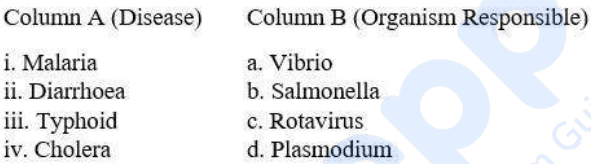
Match the points under Column A with those under Column B.
Important Questions from Measurement and Analysis of Data
Arrange the following researches in an increasing order in terms of generalization of their respective findings:
A. Ethnographic research
B. Survey research
C. Experimental research
D. Action research
E. Case study research
Choose the correct answer from the options given below:
Which of the following are not true for ANCOVA ?
A. It uses partial correlation principles.
B. It transforms quasi-experiment into a true experiment.
C. It has two dependent variables.
D. It controls variance at analysis stage.
E. It controls variance at the time of structuring research design.
Choose the correct answer from the options given below:
- The correlation coefficient between scores on two parts of a given test is 0.50. What is the reliability coefficient of the total test?
- What will be the 't value' when 'between-groups variance' and 'within-groups variance' is 200 and 50 respectively ?
For a symmetric distribution, which of the following formula is not correct?