
Fourier transform and Laplace transform are the significant mathematical tools used for signal and system analysis. The limitation of Fourier transform is that it is not defined for some of the signals. Therefore for such signals analysis Laplace transform is used to overcome the drawback of Fourier transform. Due to availability of convergence factor Laplace transform is completely integrable and hence defined for those signals for which Fourier transform is not absolutely integrable. The LTI is represented by differential equation. The system response is obtained by solving the given differential equation. Any differential equation is converted into simpler algebraic equation by Laplace transform.
Laplace transform is equivalent to Fourier transform when, the real term \((\sigma)\) of complex frequency \(S=\sigma+j\omega\) ,should be
\(\sigma=0\)
Write both transforms side by side.
Bilateral Laplace transform, with complex frequency \(s=\sigma+j\omega\):
\(X(s)=\int_{-\infty}^{\infty}x(t)e^{-st}\,dt\)
Fourier transform:
\(X(j\omega)=\int_{-\infty}^{\infty}x(t)e^{-j\omega t}\,dt\)
Compare the kernels. Substituting \(s=\sigma+j\omega\) splits the Laplace kernel into two factors:
\(e^{-st}=e^{-\sigma t}\,e^{-j\omega t}\)
The oscillating factor \(e^{-j\omega t}\) is common to both transforms. The only difference is the real exponential \(e^{-\sigma t}\), the convergence (damping) factor that Laplace adds.
Set the two equal. The transforms coincide when that extra factor becomes unity:
\(e^{-\sigma t}=1 \Rightarrow \sigma = 0 \Rightarrow s=j\omega\)
Geometric meaning. σ = 0 is the imaginary (jω) axis of the s-plane. So the Fourier transform is simply the Laplace transform evaluated along that axis — which is why one can read a system's frequency response straight off its transfer function by putting \(s=j\omega\) in H(s).
An important condition. This equivalence is valid only if the jω axis actually lies inside the region of convergence. For a stable system all poles are in the left half plane, the ROC includes the jω axis, and H(jω) exists. For an unstable system — say a pole at s = +2 — the ROC excludes the axis and the Fourier transform does not exist even though the Laplace transform does. This is exactly why Laplace is the more general tool: the damping factor \(e^{-\sigma t}\) can force convergence for signals that grow with time, such as a ramp or a rising exponential, which have no Fourier transform.
Checking the other options. σ = 1 or σ = −1 leaves a residual factor \(e^{\mp t}\) that weights the signal, and σ = ∞ would annihilate the integrand altogether.
Hence, the two transforms are equivalent when σ = 0.
Similar Questions
The Laplace transform converts integro-differential equation in _________ domain.
If \(x(t)=e^{-ct}-e^{-dt}\,u(-t)\), Laplace transform of x(t) is
For two signals \(x_1(t)\) and \(x_2(t)\). The correct Laplace transform expression for \(x_1(t)\cdot x_2(t)\) is :
Unit parabolic function is represented by its Laplace transform as:
A function f(t) is given by e–αt cos ωt. Its pole location in s-plane will be given by
Following statements are given for Laplace transforms :
(a) \(L[x(t)]=\displaystyle\int_{-\infty}^{\infty}x(t)e^{st}\,dt\)
(b) \(L[x(t)]=\displaystyle\int_{-\infty}^{\infty}x(t)e^{-st}\,dt\)
(c) \(L\left[te^{-at}u(t)\right]=\dfrac{1}{(s+a)^{2}}\)
(d) \(L\left[te^{-at}u(t)\right]=\dfrac{1}{(s-a)^{2}}\)
Out of the above, the following is the correct answer :
Match the following :
List - I List - II a) $(\dfrac{1}{s-\alpha})$ i) 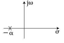
b) $(\dfrac{1}{s+\alpha})$ ii) 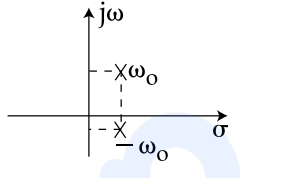
c) $(\dfrac{1}{(s-\alpha)^{2}+\omega_{o}^{2}})$ iii) 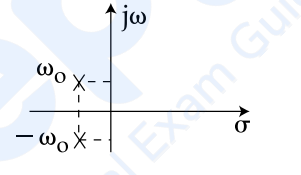
d) $(\dfrac{1}{(s+\alpha)^{2}+\omega_{o}^{2}})$ iv) 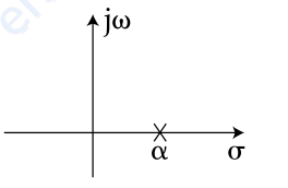
Codes :
Assertion (A) : Laplace and Z transforms can be applied to the analysis of many unstable systems and consequently play an important role in the investigation of the stability or instability of the systems.
Reason (R) : The region of convergence of the Laplace transform of x(t) is given by the expression : \(\displaystyle\int_{-\infty}^{\infty}x(t)e^{-\sigma t}\,dt\ \ge\ \infty\)
Select your answer using the codes given below :
Laplace transform of e–at sin ωt is
Fourier transform and Laplace transform are the significant mathematical tools used for signal and system analysis. The limitation of Fourier transform is that it is not defined for some of the signals. Therefore for such signals analysis Laplace transform is used to overcome the drawback of Fourier transform. Due to availability of convergence factor Laplace transform is completely integrable and hence defined for those signals for which Fourier transform is not absolutely integrable.
The LTI is represented by differential equation. The system response is obtained by solving the given differential equation. Any differential equation is converted into simpler algebraic equation by Laplace transform.
Important Questions from Laplace Transform
Which of the following is the final value of the impulse response of the system whose transfer function is
(2s + 1)/(s 4 + 8s 3 + 16s 2 + s)
Find the Laplace transform for the following time domain.
y(t) = -2te -t + 4e -t - 4e -2t
Match List I with List II
List – I
List – II
f(t)
F(S)
A.
e -at
I.
\(\rm \frac{s}{s^2+ \omega^2}\)
B.
te at
II.
\(\rm \frac{\omega}{s^2+ \omega^2}\)
C.
sinωt
III.
\(\rm \frac{1}{(s- a)^2}\)
D.
cosωt
IV.
\(\rm \frac{1}{(s+ a)}\)
Choose the correct answer from the options given below:
Laplace transform of the function f(t) denoted by F(s) is given by
What will be the Laplace transform for f(t) = e-bt u(t) ?



