
An atom is restricted to move in one dimension by making unit jumps either to the left or right, as shown in the figure. Assuming that a jump to the left or right is equally probable, the probability of the atom returning back to the starting point after four jumps is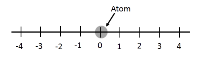
To solve the problem of finding the probability that an atom returns to its starting point after four jumps, we need to analyze the possible movements of the atom.
An atom can move left or right at each step. After four jumps, the atom will return to the starting point if it makes an equal number of left and right moves. This is because moving left cancels out moving right.
Consider the number of different ways the atom can return to the starting point:
- Two moves to the left and two moves to the right in any order.
This can be calculated using combinations. We need to select 2 moves to the left (or right) out of 4, which can be done in \(C(4,2)\) ways.
The formula for combinations is:
\(C(n, k) = \frac{n!}{k!(n-k)!}\)
Applying this formula to our problem:
\(C(4, 2) = \frac{4!}{2!(4-2)!} = \frac{4 \times 3}{2 \times 1} = 6\)
There are a total of \(2^4 = 16\) possible sequences of jumps because for each jump, there are 2 choices (left or right).
Thus, the probability that the atom returns to the starting point is:
\(\frac{6}{16} = 0.375\)
Therefore, the probability of the atom returning to the starting point after four jumps is 0.375.
Important Questions from Discrete Distributions
The value of a and b so that the following is probability mass function
X: 0 1 2 P(X = x): 3a 3b 4b with mean 1.1, is:
Digital data received from a sensor can fill up 0 to 32 buffers. Let the sample space be
S = {0, 1, 2, .........., 32} where the sample j denote that j of the buffers are full and \(p\left( i \right) = \frac{1}{{561}}\left( {33 - i} \right)\)
. Let A denote the event that the even number of buffers are full. Then p(A) is :If X is a Poisson random variate with mean 3, then P(|X- 3| < 1) will be:
Let x ∼ N(μ, σ2) If μ2 = σ2, (μ > 0), then the value of P(X < -μ | X < μ) in terms of cumulative function N (0, 1) is:
Consider a binomial random variable X. If X1, X2,...Xn are independent and identically distributed samples from the distribution of X with sum \(Y = \mathop \sum \limits_{i = 1}^n {X_i}\) then the distribution of Y as n → ∞ can be approximated as.


